|
If you have a set of interesting Affy probes or genes that you'd like to annotate, you can build a simple tool in Excel
that will let you gather information about these probes in an attempt to explain what they have in common or what physiological
significance they may have.
Annotation is easy with an Affy chip, since Affymetrix has assembled data from a variety of sources for all probesets of their chips.
If you're using a custom array or one by another manufacturer, you may have to generate the annotation file yourself.
The process shown shown below is for Affy chips, so the first step ("Getting the annotation file") may vary for other types of chips.
A sample tool can be downloaded as a zipped Excel file or
an Excel file. It may be easier to start with this sample file, instead of building your file from scratch.
This is somewhat different from the description (below), in that two different worksheets are used. In this case, you need to know the notation for
referrring to another worksheet. For example, in the formula
=VLOOKUP($A2,anno!$A$2:$J$14011,2,FALSE)
"anno!$A$2:$J$14011" refers to cells $A$2:$J$14011 on worksheet anno.
Getting the annotation file
- If you're not using an Affy chip, get the annotation file from the manufacturer or create it yourself.
- If you're using an Affy chip, go to the Affymetrix Support site.
- Select an array and go to that page.
- Under "NetAffx Annotation Files," click on the "CSV" link.
- You'll be prompted to log in to the system (or register for free).
- Save the .zip file on your computer and then unzip it.
Editing the annotation file in Excel
- Open the .csv ("comma-separated value") file in Excel.
- Examine all of the data fields in the file.
- Delete all of the columns that aren't very informative.
For example, the fields "Chip," "Organism," and "Annotation Date" can be recorded somewhere but then deleted, since they're the same for all rows.
- Save the file as a standard Excel file (.xls for Windows), since you'll be using formulas that can't be saved in .csv format.
Creating the annotation columns
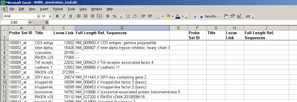
- To the right of the annotation columns, add another set of column headings:

- The idea is that you'll paste a list of probes in the "Probe set ID" column on the right, and Excel will fill in the rest of the columns for those probes.
Writing the Excel formulas
- You'll be entering formulas in the first row of cells in your column (cells G2, H2, and I2 in the figure above)- except the first column where you paste the probe IDs - so Excel can find the corresponding information.
These formulas can then be pasted in other rows.
- The key formula you'll be using is VLOOKUP. At any time, you can look for VLOOKUP in the Excel help for more information and examples.
- Another key Excel convention is the use of the '$' prefix to show a cell that is constant even when the formula is copied and pasted.
Example: If a formula in row 2 referring to cell A2 is pasted into row 3, the formula will now refer to cell A3.
If a formula in row 2 referring to cell $A$2 is pasted into row 3, the formula will still refer to cell A2.
- In the first cell to the right of the probe ID (input data) column (F2 above), enter the following formula:
=VLOOKUP(input,dataTopLeft:dataBottomRight,colNum,FALSE)
with the following information:
- input = input cell for this row (F2 in the figure above), with the column made constant ($F2)
- dataTopLeft = top left cell for the columns containing all the annotation data (A2 in the figure above), made constant ($A$2).
- dataBottomRight = bottom right cell for the columns containing all the annotation data (D12423 for the array above), made constant ($D$12423).
- colNum = column number containing data to put in this cell (4 in the example above, since the "title" data that you want in this column
is found in column 2 of the annotation data).
- FALSE: since you want VLOOKUP to find only an exact match
An example for the Excel file above is
=VLOOKUP($F2,$A$2:$D$12423,2,FALSE)
- Paste a probe into the "input" cell to the right and check that the formula works. In the example below, using "10001_at" as input,
the formula could find the corresponding Title:

- In the second cell to the right of the probe ID (input data) column (F2 above), enter a similar formula, replacing colNum:
=VLOOKUP($F2,$A$2:$D$12423,3,FALSE)

- For the rest of the cells in the first row of the "output" section, enter similar formulas, always replacing colNum with the appropriate number.
- Copy all the cells where you entered formulas and paste them into rows below - as many rows as you expect to have input genes in your lists.
In the example, cells G2, H2, and I2 were pasted into rows 3 - 101 (if my probe ID lists were as long as 100 entries)

- After pasting the cells with formulas, the file will look something like this:

All of the #N/A will remain until probe set IDs are pasted into the input column.
- Try pasting a column of probe set IDs to check that everything works.
- You can even add hyperlinks to web pages, such as those for NCBI's LocusLink or Unigene.
For example, if you already have the LocusLink ID, use a formula like
=HYPERLINK(CONCATENATE("http://www.ncbi.nlm.nih.gov/LocusLink/LocRpt.cgi?l=", H2))
to make a link to the LocusLink page for the LocusLink ID in cell H2.
Helpful equations
- Using IF and ISNA:
=IF(ISNA(VLOOKUP(input,dataTopLeft:dataBottomRight,colNum,FALSE)), VLOOKUP(input,dataTopLeft:dataBottomRight,colNum,FALSE), "alternate message")
- Referring to other worksheets (in this case, a sheet named "NOTES"):
=IF(ISNA(VLOOKUP(A2,NOTES!$B$1:NOTES!$C$100,2,FALSE)), "", "EXPIRED")
|


